
Reading: Wooldridge Ch 7
- Using the data on individuals’ time use, we estimate the equation
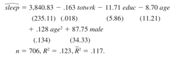
The variable sleep is total minutes per week spent sleeping at night, totwrk is total weekly minutes spent working, educ and age are measured in years, and male is a gender dummy.
(i) All other factors being equal, is there evidence that men sleep more than women?
How strong is the evidence?
(ii) Is there a statistically significant tradeoff between working and sleeping? What is
the estimated tradeoff?
(iii) What other regression do you need to run to test the null hypothesis that, holding
other factors fixed, age has no effect on sleeping?
- An equation explaining chief executive officer salary is estimated to be
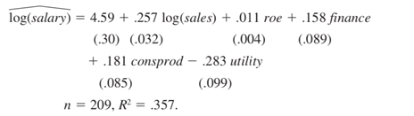
where finance, consprod, and utility are binary variables indicating the financial, consumer products, and utilities industries. The omitted industry is transportation.
(i) Compute the approximate percentage difference in estimated salary between the utility and transportation industries, holding sales and roe fixed. Is the difference statistically significant at the 1% level?
(ii) Use equation (7.10) to obtain the exact percentage difference in estimated salary between the utility and transportation industries and compare this with the answer obtained in part (i).
(iii) What is the approximate percentage difference in estimated salary between the consumer products and finance industries? Write an equation that would allow you to test whether the difference is statistically significant.
- Use the data set BEAUTY, which contains a subset of the variables reported by Hamermesh and Biddle (1994).
(i) Find the separate fractions of men and women that are classified as having above aver-
age looks. Are more people rated as having above average or below average looks?
(ii) Test the null hypothesis that the population fractions of above-average-looking women and men are the same. Report the one-sided p-value that the fraction is
higher for women. (Hint: Estimating a simple linear probability model is easiest.)
(iii) Now estimate the model

separately for men and women, and report the results in the usual form. In both cases, interpret the coefficient on belavg. Explain in words what the null hypothesis H0: β1=0 against H1: β1<0 means, and find the p-values for men and women.
(iv) Is there convincing evidence that women with above average looks earn more than women with average looks? Explain.
(v) For both men and women, add the explanatory variables educ, exper, exper2, union, goodhlth, black, married, south, bigcity, smllcity, and service. Do the effects of the “looks” variables change in important ways?